
All in One View
Content from Why use a Cluster?
Last updated on 2026-09-15 | Edit this page
Overview
Questions
- Why would I be interested in High-Performance Computing (HPC)?
- What can I expect to learn from this course?
Objectives
- Describe what an HPC system is
- Identify how an HPC system could benefit you.
Frequently, research problems that use computing can outgrow the capabilities of the desktop or laptop computer where they started:
- A statistics student wants to cross-validate a model. This involves running the model 1000 times — but each run takes an hour. Running the model on a laptop will take over a month! In this research problem, final results are calculated after all 1000 models have run, but typically only one model is run at a time (in serial) on the laptop. Since each of the 1000 runs is independent of all others, and given enough computers, it’s theoretically possible to run them all at once (in parallel).
- A genomics researcher has been using small datasets of sequence data, but soon will be receiving a new type of sequencing data that is 10 times as large. It’s already challenging to open the datasets on a computer — analyzing these larger datasets will probably crash it. In this research problem, the calculations required might be impossible to parallelize, but a computer with more memory would be required to analyze the much larger future data set.
- An engineer is using a fluid dynamics package that has an option to run in parallel. So far, this option was not used on a desktop. In going from 2D to 3D simulations, the simulation time has more than tripled. It might be useful to take advantage of that option or feature. In this research problem, the calculations in each region of the simulation are largely independent of calculations in other regions of the simulation. It’s possible to run each region’s calculations simultaneously (in parallel), communicate selected results to adjacent regions as needed, and repeat the calculations to converge on a final set of results. In moving from a 2D to a 3D model, both the amount of data and the amount of calculations (the number of computations) increases greatly, and it’s theoretically possible to distribute the calculations across multiple computers (nodes) communicating over a shared network.
In all these cases, access to more (and larger) computers is needed. Those computers should be usable at the same time, solving many researcher’s problems in parallel.
Jargon Busting Presentation
Open the HPC Jargon Buster in a
new tab. To present the content, press C to open a
clone in a separate window, then press P
to toggle presentation mode.
I’ve Never Used a Server, Have I?
Take a minute and think about which of your daily interactions with a computer may require a remote server or even cluster to provide you with results.
- Checking email: your computer (possibly in your pocket) contacts a remote machine, authenticates, and downloads a list of new messages; it also uploads changes to message status, such as whether you read, marked as junk, or deleted the message. Since yours is not the only account, the mail server is probably one of many in a data center.
- Searching for a phrase online involves comparing your search term against a massive database of all known sites, looking for matches. This “query” operation can be straightforward, but building that database is a monumental task! Servers are involved at every step.
- Searching for directions on a mapping website involves connecting your (A) starting and (B) end points by traversing a graph in search of the “shortest” path by distance, time, expense, or another metric. Converting a map into the right form is relatively simple, but calculating all the possible routes between A and B is expensive.
Checking email could be serial: your machine connects to one server and exchanges data. Searching by querying the database for your search term (or endpoints) could also be serial, in that one machine receives your query and returns the result. However, assembling and storing the full database is far beyond the capability of any one machine. Therefore, these functions are served in parallel by a large, “hyperscale” collection of servers working together.
- High-Performance Computing (HPC) typically involves connecting to very large computing systems elsewhere in the world.
- These other systems can be used to do work that would either be impossible or much slower on smaller systems.
- HPC resources are shared by multiple users.
- The standard method of interacting with such systems is via a command line interface.
Content from Working on a remote HPC system
Last updated on 2026-09-15 | Edit this page
Overview
Questions
- “What is an HPC system?”
- “How does an HPC system work?”
- “How do I log on to a remote HPC system?”
Objectives
- “Connect to a remote HPC system.”
- “Understand the general HPC system architecture.”
What Is an HPC System?
The words “cloud”, “cluster”, and the phrase “high-performance computing” or “HPC” are used a lot in different contexts and with various related meanings. So what do they mean? And more importantly, how do we use them in our work?
The cloud is a generic term commonly used to refer to computing resources that are a) provisioned to users on demand or as needed and b) represent real or virtual resources that may be located anywhere on Earth. For example, a large company with computing resources in Brazil, Zimbabwe and Japan may manage those resources as its own internal cloud and that same company may also utilize commercial cloud resources provided by Amazon or Google. Cloud resources may refer to machines performing relatively simple tasks such as serving websites, providing shared storage, providing web services (such as e-mail or social media platforms), as well as more traditional compute intensive tasks such as running a simulation.
The term HPC system, on the other hand, describes a stand-alone resource for computationally intensive workloads. They are typically comprised of a multitude of integrated processing and storage elements, designed to handle high volumes of data and/or large numbers of floating-point operations (FLOPS) with the highest possible performance. For example, all of the machines on the Top-500 list are HPC systems. To support these constraints, an HPC resource must exist in a specific, fixed location: networking cables can only stretch so far, and electrical and optical signals can travel only so fast.
The word cluster is often used for small to moderate scale HPC resources less impressive than the Top-500. Clusters are often maintained in computing centers that support several such systems, all sharing common networking and storage to support common compute intensive tasks.
Logging In
The first step in using a cluster is to establish a connection from our laptop to the cluster. When we are sitting at a computer (or standing, or holding it in our hands or on our wrists), we have come to expect a visual display with icons, widgets, and perhaps some windows or applications: a graphical user interface, or GUI. Since computer clusters are remote resources that we connect to over often slow or laggy interfaces (WiFi and VPNs especially), it is more practical to use a command-line interface, or CLI, in which commands and results are transmitted via text, only. Anything other than text (images, for example) must be written to disk and opened with a separate program.
If you have ever opened the Windows Command Prompt or macOS Terminal, you have seen a CLI. If you have already taken “The Carpentries” courses on the UNIX Shell or Version Control, you have used the CLI on your local machine somewhat extensively. The only leap to be made here is to open a CLI on a remote machine, while taking some precautions so that other folks on the network can’t see (or change) the commands you’re running or the results the remote machine sends back. We will use the Secure Shell protocol (or SSH) to open an encrypted network connection between two machines, allowing you to send & receive text and data without having to worry about prying eyes.
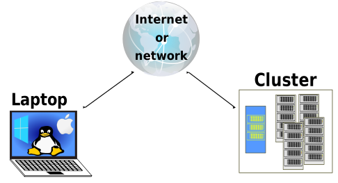
Make sure you have a SSH client installed on your laptop. Refer to
the setup section for more details. SSH clients
are usually command-line tools, where you provide the remote machine
address as the only required argument. If your username on the remote
system differs from what you use locally, you must provide that as well.
If your SSH client has a graphical front-end, such as PuTTY or
MobaXterm, you will set these arguments before clicking “connect.” From
the terminal, you’ll write something like
ssh username@hostname, where the “@” symbol is used to
separate the two parts of a single argument.
Go ahead and open your terminal or graphical SSH client, then log in to the cluster using your username and the remote computer you can reach from the outside world, comet.ncl.ac.uk.
Remember to replace user with your username or the one
supplied by the instructors. You may be asked for your password. Watch
out: the characters you type after the password prompt are not displayed
on the screen. Normal output will resume once you press
Enter.
Where Are We?
Very often, many users are tempted to think of a high-performance
computing installation as one giant, magical machine. Sometimes, people
will assume that the computer they’ve logged onto is the entire
computing cluster. So what’s really happening? What computer have we
logged on to? The name of the current computer we are logged onto can be
checked with the hostname command. (You may also notice
that the current hostname is also part of our prompt!)
OUTPUT
cometlogin01What’s in Your Home Directory?
The system administrators may have configured your home directory
with some helpful files, folders, and links (shortcuts) to space
reserved for you on other filesystems. Take a look around and see what
you can find. Hint: The shell commands pwd and
ls may come in handy. Home directory contents vary from
user to user. Please discuss any differences you spot with your
neighbors.
The deepest layer should differ: user is uniquely yours.
Are there differences in the path at higher levels?
If both of you have empty directories, they will look identical. If you or your neighbor has used the system before, there may be differences. What are you working on?
Use pwd to print the
working directory path:
You can run ls to list
the directory contents, though it’s possible nothing will show up (if no
files have been provided). To be sure, use the -a flag to
show hidden files, too.
At a minimum, this will show the current directory as .,
and the parent directory as ...
Nodes
Individual computers that compose a cluster are typically called nodes (although you will also hear people call them servers, computers and machines). On a cluster, there are different types of nodes for different types of tasks. The node where you are right now is called the head node, login node, landing pad, or submit node. A login node serves as an access point to the cluster.
As a gateway, it is well suited for uploading and downloading files, setting up software, and running quick tests. Generally speaking, the login node should not be used for time-consuming or resource-intensive tasks. You should be alert to this, and check with your site’s operators or documentation for details of what is and isn’t allowed. In these lessons, we will avoid running jobs on the head node.
Dedicated Transfer Nodes
If you want to transfer larger amounts of data to or from the cluster, some systems offer dedicated nodes for data transfers only. The motivation for this lies in the fact that larger data transfers should not obstruct operation of the login node for anybody else. Check with your cluster’s documentation or its support team if such a transfer node is available. As a rule of thumb, consider all transfers of a volume larger than 500 MB to 1 GB as large. But these numbers change, e.g., depending on the network connection of yourself and of your cluster or other factors.
The real work on a cluster gets done by the worker (or compute) nodes. Worker nodes come in many shapes and sizes, but generally are dedicated to long or hard tasks that require a lot of computational resources.
All interaction with the worker nodes is handled by a specialized piece of software called a scheduler (the scheduler used in this lesson is called Slurm). We’ll learn more about how to use the scheduler to submit jobs next, but for now, it can also tell us more information about the worker nodes.
For example, we can view all of the worker nodes by running the
command sinfo.
OUTPUT
PARTITION          AVAIL  TIMELIMIT  NODES  STATE NODELIST
cpubase_bycore_b1*    up   infinite      4   idle node[1-2],smnode[1-2]
node                  up   infinite      2   idle node[1-2]
smnode                up   infinite      2   idle smnode[1-2]
There are also specialized machines used for managing disk storage, user authentication, and other infrastructure-related tasks. Although we do not typically logon to or interact with these machines directly, they enable a number of key features like ensuring our user account and files are available throughout the HPC system.
What's in a Node?
All of the nodes in an HPC system have the same components as your own laptop or desktop: CPUs (sometimes also called processors or cores), memory (or RAM), and disk space. CPUs are a computer’s tool for actually running programs and calculations. Information about a current task is stored in the computer’s memory. Disk refers to all storage that can be accessed like a filesystem. This is generally storage that can hold data permanently, i.e. data is still there even if the computer has been restarted. While this storage can be local (a hard drive installed inside of it), it is more common for nodes to connect to a shared, remote fileserver or cluster of servers.
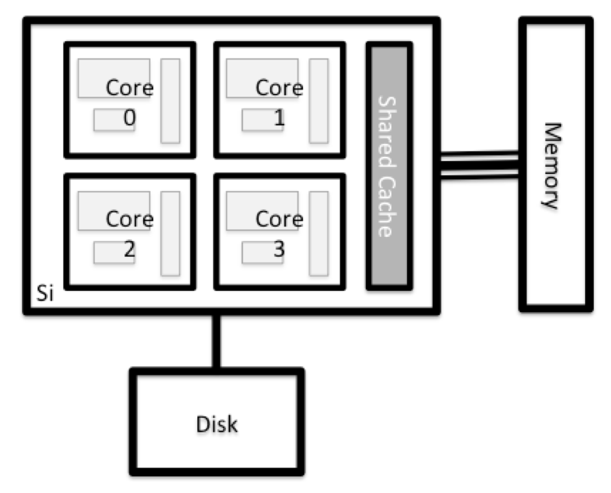
There are several ways to do this. Most operating systems have a graphical system monitor, like the Windows Task Manager. More detailed information can sometimes be found on the command line. For example, some of the commands used on a Linux system are:
Run system utilities
Read from /proc
Use a system monitor
Explore the login node
Now compare the resources of your computer with those of the head node.
BASH
[you@laptop:~]$ ssh user@comet.ncl.ac.uk
[user@cometlogin01(comet) ~] nproc --all
[user@cometlogin01(comet) ~] free -m
You can get more information about the processors using
lscpu, and a lot of detail about the memory by reading the
file /proc/meminfo:
You can also explore the available filesystems using df
to show disk free space. The
-h flag renders the sizes in a human-friendly format, i.e.,
GB instead of B. The type flag -T shows
what kind of filesystem each resource is.
The local filesystems (ext, tmp, xfs, zfs) will depend on whether
you’re on the same login node (or compute node, later on). Networked
filesystems (beegfs, cifs, gpfs, nfs, pvfs) will be similar — but may
include /usr, depending on how it is mounted.
Compare Your Computer, the login node and the compute node
Compare your laptop’s number of processors and memory with the numbers you see on the cluster head node and worker node. Discuss the differences with your neighbor.
What implications do you think the differences might have on running your research work on the different systems and nodes?
Differences Between Nodes
Many HPC clusters have a variety of nodes optimized for particular workloads. Some nodes may have larger amount of memory, or specialized resources such as Graphics Processing Units (GPUs).
With all of this in mind, we will now cover how to talk to the cluster’s scheduler, and use it to start running our scripts and programs!
- An HPC system is a set of networked machines.
- HPC systems typically provide login nodes and a set of worker nodes.
- The resources found on independent (worker) nodes can vary in volume and type (amount of RAM, processor architecture, availability of network-mounted filesystems, etc.).
- Files saved on one node are typically accessible from all nodes via a shared filesystem.
Content from Scheduler Fundamentals
Last updated on 2026-09-15 | Edit this page
Overview
Questions
- What is a scheduler and why does a cluster need one?
- How do I launch a program to run on a compute node in the cluster?
- How do I capture the output of a program that is run on a node in the cluster?
Objectives
- Submit a simple script to the cluster.
- Monitor the execution of jobs using command line tools.
- Inspect the output and error files of your jobs.
- Find the right place to put large datasets on the cluster.
Job Scheduler
An HPC system might have thousands of nodes and thousands of users. How do we decide who gets what and when? How do we ensure that a task is run with the resources it needs? This job is handled by a special piece of software called the scheduler. On an HPC system, the scheduler manages which jobs run where and when.
The following illustration compares these tasks of a job scheduler to a waiter in a restaurant. If you can relate to an instance where you had to wait for a while in a queue to get in to a popular restaurant, then you may now understand why sometimes your job do not start instantly as in your laptop.
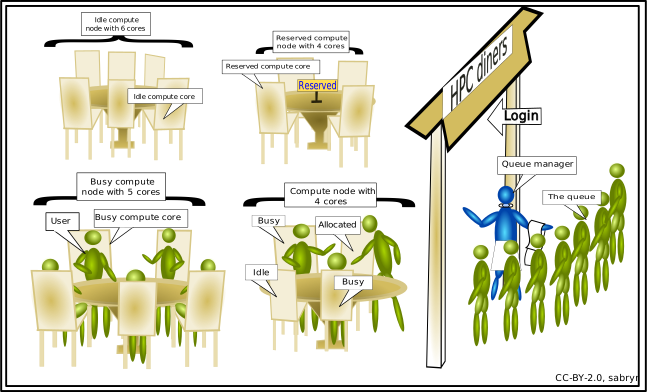
The scheduler used in this lesson is Slurm. Although Slurm is not used everywhere, running jobs is quite similar regardless of what software is being used. The exact syntax might change, but the concepts remain the same.
Running a Batch Job
The most basic use of the scheduler is to run a command non-interactively. Any command (or series of commands) that you want to run on the cluster is called a job, and the process of using a scheduler to run the job is called batch job submission.
In this case, the job we want to run is a shell script – essentially a text file containing a list of UNIX commands to be executed in a sequential manner. Our shell script will have three parts:
- On the very first line, add
#!/bin/bash. The#!(pronounced “hash-bang” or “shebang”) tells the computer what program is meant to process the contents of this file. In this case, we are telling it that the commands that follow are written for the command-line shell (what we’ve been doing everything in so far). - Anywhere below the first line, we’ll add an
echocommand with a friendly greeting. When run, the shell script will print whatever comes afterechoin the terminal.-
echo -nwill print everything that follows, without ending the line by printing the new-line character.
-
- On the last line, we’ll invoke the
hostnamecommand, which will print the name of the machine the script is run on.
Creating Our Test Job
Run the script. Does it execute on the cluster or just our login node?
This script ran on the login node, but we want to take advantage of
the compute nodes: we need the scheduler to queue up
example-job.sh to run on a compute node.
To submit this task to the scheduler, we use the sbatch
command. This creates a job which will run the script
when dispatched to a compute node which the queuing system has
identified as being available to perform the work.
OUTPUT
Submitted batch job 7And that’s all we need to do to submit a job. Our work is done – now
the scheduler takes over and tries to run the job for us. While the job
is waiting to run, it goes into a list of jobs called the
queue. To check on our job’s status, we check the queue using
the command squeue -u yourUsername.
OUTPUT
JOBID PARTITION     NAME     USER ST       TIME  NODES NODELIST(REASON)
    9 cpubase_b example-   user01  R       0:05      1 node1
We can see all the details of our job, most importantly that it is in
the R or RUNNING state. Sometimes our jobs
might need to wait in a queue (PENDING) or have an error
(E).
Where’s the Output?
On the login node, this script printed output to the terminal – but
now, when squeue shows the job has finished, nothing was
printed to the terminal.
Cluster job output is typically redirected to a file in the directory
you launched it from. Use ls to find and cat
to read the file.
Customising a Job
The job we just ran used all of the scheduler’s default options. In a real-world scenario, that’s probably not what we want. The default options represent a reasonable minimum. Chances are, we will need more cores, more memory, more time, among other special considerations. To get access to these resources we must customize our job script.
Comments in UNIX shell scripts (denoted by #) are
typically ignored, but there are exceptions. For instance the special
#! comment at the beginning of scripts specifies what
program should be used to run it (you’ll typically see
#!/usr/bin/env bash). Schedulers like Slurm also have a
special comment used to denote special scheduler-specific options.
Though these comments differ from scheduler to scheduler, Slurm’s
special comment is #SBATCH. Anything following the
#SBATCH comment is interpreted as an instruction to the
scheduler.
Let’s illustrate this by example. By default, a job’s name is the
name of the script, but the --job-name option can be used
to change the name of a job. Add an option to the script:
Submit the job and monitor its status:
BASH
[user@cometlogin01(comet) ~] sbatch --account=comet_training example-job.sh
[user@cometlogin01(comet) ~] squeue -u yourUsername
OUTPUT
JOBID PARTITION     NAME     USER ST       TIME  NODES NODELIST(REASON)
   10 cpubase_b hello-wo   user01  R       0:02      1 node1
Fantastic, we’ve successfully changed the name of our job!
Resource Requests
What about more important changes, such as the number of CPUs and the amount of memory required for our jobs? One thing that is absolutely critical when working on an HPC system is specifying the resources required to run a job. This allows the scheduler to find suitable resources and schedule the job effectively. If you do not specify requirements (such as the amount of time you need), you will likely be assigned your site’s default resources, which is probably not what you want.
The following are several key resource requests:
--ntasks=<number>or-n <number>: How many parallel tasks (typically MPI ranks or processes) should Slurm launch?--ntasks-per-node=<ntasks>: How many tasks should be launched on each compute node?--cpus-per-task=<ncpus>or-c <ncpus>: How many CPUs should be allocated to each task/process?--partition=<partition>or-p <partition>: Specify which scheduler partition/queue the job should run in.--time=<days-hours:minutes:seconds>or-t <days-hours:minutes:seconds>: How much real-world time (walltime) will your job take to run? The<days>part can be omitted.-
--mem=<size>[units]: How much memory should be allocated per node for your job? Memory units may be specified using the following suffixes:-
Korkfor kilobytes -
Mormfor megabytes -
Gorgfor gigabytes -
Tortfor terabytes Example:--mem=5Gor--mem=5g
-
--mem-per-cpu=<size>[units]: How much memory should be allocated per CPU? This is commonly used on shared-node systems where memory allocation is tied to CPU allocation.--nodes=<nnodes>or-N <nnodes>: How many compute nodes should be allocated for your job? Note that if the requestedntaskscount cannot fit within available resources of one node, Slurm may allocate multiple nodes automatically, subject to partition limits and scheduler policies.
For some resources, such as GPUs, the way to request them may be site-specific or specific to version of the resource scheduler. For this reason we do not include them in the list above.
Note that just requesting these resources does not make your job run faster, nor does it necessarily mean that you will consume all of these resources. It only means that these are made available to you. Your job may end up using less memory, or less time, or fewer nodes than you have requested, and it will still run.
It’s best if your requests accurately reflect your job’s requirements. We’ll talk more about how to make sure that you’re using resources effectively in a later episode of this lesson.
Submitting Resource Requests
Modify our hostname script so that it runs for a minute,
then submit a job for it on the cluster.
Resource requests are typically binding. If you exceed them, your job will be killed. Let’s use wall time as an example. We will request 1 minute of wall time, and attempt to run a job for two minutes.
BASH
#!/bin/bash
#SBATCH --job-name long_job
#SBATCH --time 00:01 # timeout in HH:MM

echo "This script is running on ... "
sleep 240 # time in seconds
hostname
Submit the job and wait for it to finish. Once it is has finished, check the log file.
BASH
[user@cometlogin01(comet) ~] sbatch --account=comet_training example-job.sh
[user@cometlogin01(comet) ~] squeue -u yourUsernameOUTPUT
This script is running on ...
slurmstepd: error: *** JOB 12 ON node1 CANCELLED AT 2021-02-19T13:55:57
DUE TO TIME LIMIT ***
Our job was killed for exceeding the amount of resources it requested. Although this appears harsh, this is actually a feature. Strict adherence to resource requests allows the scheduler to find the best possible place for your jobs. Even more importantly, it ensures that another user cannot use more resources than they’ve been given. If another user messes up and accidentally attempts to use all of the cores or memory on a node, Slurm will either restrain their job to the requested resources or kill the job outright. Other jobs on the node will be unaffected. This means that one user cannot mess up the experience of others, the only jobs affected by a mistake in scheduling will be their own.
Cancelling a Job
Sometimes we’ll make a mistake and need to cancel a job. This can be
done with the scancel command. Let’s submit a job and then
cancel it using its job number (remember to change the walltime so that
it runs long enough for you to cancel it before it is killed!).
BASH
[user@cometlogin01(comet) ~] sbatch --account=comet_training example-job.sh
[user@cometlogin01(comet) ~] squeue -u yourUsername
OUTPUT
Submitted batch job 13

JOBID PARTITION     NAME     USER ST       TIME  NODES NODELIST(REASON)
   13 cpubase_b long_job   user01  R       0:02      1 node1
Now cancel the job with its job number (printed in your terminal). A clean return of your command prompt indicates that the request to cancel the job was successful.
BASH
[user@cometlogin01(comet) ~] scancel 38759
# It might take a minute for the job to disappear from the queue...
[user@cometlogin01(comet) ~] squeue -u yourUsername
OUTPUT
JOBID PARTITION NAME USER ST TIME NODES NODELIST(REASON)Cancelling multiple jobs
We can also cancel all of our jobs at once using the -u
option. This will delete all jobs for a specific user (in this case,
yourself). Note that you can only delete your own jobs.
Try submitting multiple jobs and then cancelling them all.
Other Types of Jobs
Up to this point, we’ve focused on running jobs in batch mode.
Slurm also provides the ability to start an interactive
session.
There are very frequently tasks that need to be done interactively.
Creating an entire job script might be overkill, but the amount of
resources required is too much for a login node to handle. A good
example of this might be building a genome index for alignment with a
tool like HISAT2.
Fortunately, we can run these types of tasks as a one-off with
srun.
srun runs a single command on the cluster and then
exits. Let’s demonstrate this by running the hostname
command with srun. (We can cancel an srun job
with Ctrl-c.)
OUTPUT
compute030srun accepts all of the same options as
sbatch. However, instead of specifying these in a script,
these options are specified on the command-line when starting a job. To
submit a job that uses 2 CPUs for instance, we could use the following
command:
OUTPUT
This job will use 2 CPUs.
This job will use 2 CPUs.
Typically, the resulting shell environment will be the same as that
for sbatch.
Interactive jobs
Sometimes, you will need a lot of resources for interactive use.
Perhaps it’s our first time running an analysis or we are attempting to
debug something that went wrong with a previous job. Fortunately, Slurm
makes it easy to start an interactive job with srun:
You should be presented with a bash prompt. Note that the prompt will
likely change to reflect your new location, in this case the compute
node we are logged on. You can also verify this with
hostname.
Creating remote graphics
On many HPCsystems, you need to use X11 forwarding to see graphical output inside your jobs.
Because Comet has Open OnDemand installed, you should NOT use X11 forwarding in most cases. Instead launch an interactive application or desktop at https://ood01.comet.hpc.ncl.ac.uk/
When you are done with the interactive job, log out to quit your session.
- The scheduler handles how compute resources are shared between users.
- A job is just a shell script.
- Request slightly more resources than you will need.
- For interactive sessions, use
srun - For graphical interactive sessions, use Open OnDemand
Content from Environment Variables
Last updated on 2026-09-15 | Edit this page
Overview
Questions
- How are variables set and accessed in the Unix shell?
- How can I use variables to change how a program runs?
Objectives
- Understand how variables are implemented in the shell
- Read the value of an existing variable
- Create new variables and change their values
- Change the behaviour of a program using an environment variable
- Explain how the shell uses the
PATHvariable to search for executables
Episode provenance
This episode has been remixed from the Shell Extras episode on Shell Variables and the HPC Shell episode on scripts.
The shell is just a program, and like other programs, it has variables. Those variables control its execution, so by changing their values you can change how the shell behaves (and with a little more effort how other programs behave).
Variables are a great way of saving information under a name you can access later. In programming languages like Python and R, variables can store pretty much anything you can think of. In the shell, they usually just store text. The best way to understand how they work is to see them in action.
Let’s start by running the command set and looking at
some of the variables in a typical shell session:
OUTPUT
...
HOME=/user
HOSTNAME=cometlogin01
HOSTTYPE=x86_64
PATH=/user/bin:/usr/local/bin:/usr/bin:/usr/local/sbin:/usr/sbin
PWD=/user
UID=1000
USER=user
...
As you can see, there are quite a few — in fact, four or five times
more than what’s shown here. And yes, using set to
show things might seem a little strange, even for Unix, but if
you don’t give it any arguments, it might as well show you things you
could set.
Every shell variable has a name and stores its value as text
(strings), even variables like UID
User ID that appear numeric.
Programs that use these variables may convert the string value into
another type when needed. For example, a program can read the value of
UID, convert it from a string to an integer user ID, look
up the corresponding username in the system user database, and return
the username as a string. The command id -un performs this
lookup automatically.
Showing the Value of a Variable
Let’s show the value of the variable HOME:
OUTPUT
HOMEThat just prints “HOME”, which isn’t what we wanted (though it is what we actually asked for). Let’s try this instead:
OUTPUT
/userThe dollar sign tells the shell that we want the value of
the variable rather than its name. This works just like wildcards: the
shell does the replacement before running the program we’ve
asked for. Thanks to this expansion, what we actually run is
echo /user, which displays the right thing.
Creating and Changing Variables
Creating a variable is easy — we just assign a value to a name using
“=” (we just have to remember that the syntax requires that there are
no spaces around the =!):
OUTPUT
DraculaTo change the value, just assign a new one:
OUTPUT
CamillaEnvironment variables
When we ran the set command we saw there were a lot of
variables whose names were in upper case. That’s because, by convention,
variables that are also available to use by other programs are
given upper-case names. Such variables are called environment
variables as they are shell variables that are defined for the
current shell and are inherited by any child shells or processes.
To create an environment variable you need to export a
shell variable. For example, to make our SECRET_IDENTITY
available to other programs that we call from our shell we can do:
You can also create and export the variable in a single step:
Using environment variables to change program behaviour
Set a shell variable TIME_STYLE to have a value of
iso and check this value using the echo
command.
Now, run the command ls with the option -l
(which gives a long format).
export the variable and rerun the ls -l
command. Do you notice any difference?
The TIME_STYLE variable is not seen by
ls until is exported, at which point it is used by
ls to decide what date format to use when presenting the
timestamp of files.
You can see the complete set of environment variables in your current
shell session with the command env (which returns a subset
of what the command set gave us). The complete set
of environment variables is called your runtime environment and
can affect the behaviour of the programs you run.
Job environment variables
When Slurm runs a job, it sets a number of environment
variables for the job. One of these will let us check what directory our
job script was submitted from. The SLURM_SUBMIT_DIR
variable is set to the directory from which our job was submitted. Using
the SLURM_SUBMIT_DIR variable, modify your job so that it
prints out the location from which the job was submitted.
To remove a variable or environment variable you can use the
unset command, for example:
The PATH Environment Variable
Similarly, some environment variables (like PATH) store
lists of values. In this case, the convention is to use a colon ‘:’ as a
separator. If a program needs the individual elements of such a list,
it’s the program’s responsibility to split the variable’s string value
into separate pieces.
Let’s take a closer look at that PATH variable. Its
value defines the shell’s search path for executables; i.e., the list of
directories the shell searches for runnable programs after you type a
command name without specifying its full path.
For example, when we type a command like bash, the shell
needs to decide which executable to run. The rule it follows is simple:
the shell checks each directory listed in PATH, in order,
looking for a program with the requested name. As soon as it finds a
match, it stops searching and executes the program.
To show how this works, here are the components of PATH
listed one per line:
OUTPUT
/user/bin
/usr/local/bin
/usr/bin
/usr/local/sbin
/usr/sbin
On our computer, there is a program called bash located
at: /usr/bin/bash. Since the shell searches the directories
in PATH in the order they are listed, it finds
/usr/bin/bash and runs it. If a program is stored in a
directory that is not listed in PATH, the shell will not
find it unless we explicitly provide the program’s full path.
This means that we can keep executables in many different locations,
as long as we update PATH so that the shell knows where to
search for them.
What if we want to run two different versions of the same program?
Since both executables share the same name, if we add both of their
directories to PATH, the version found first will always
take precedence. In the next episode, we’ll learn how to use helper
tools to manage our runtime environment more effectively, allowing us to
switch between different software versions without manually keeping
track of the value of PATH and other important environment
variables.
Modifying your PATH
Create a directory called bin in your home directory (if
it doesn’t already exist) and add it to the front of your
PATH variable. Verify that your change has been made by
displaying the contents of your PATH variable. Create a
script called hello.sh in your new bin
directory that prints “Hello, World!” to the terminal. Make the script
executable and run it from any location in your terminal.
BASH
mkdir -p ~/bin
echo '#!/bin/bash' > ~/bin/hello.sh
echo 'echo "Hello, World!"' >> ~/bin/hello.sh
chmod +x ~/bin/hello.sh
To update the PATH variable to include your new
bin directory at the front, you can do:
It is extremely important to retain the current content of
PATH by appending :$PATH to the new value;
otherwise, you will overwrite your existing PATH. This is
especially important on HPC systems, where the module load
command relies on modifying the PATH variable to make
software available to you.
Now, verify that your PATH variable has been
updated:
You should be able to run hello.sh from any location in
your terminal.
- Shell variables are by default treated as strings
- Variables are assigned using “
=” and recalled using the variable’s name prefixed by “$” - Use “
export” to make an variable available to other programs - The
PATHvariable defines the shell’s search path
Content from Accessing software via Modules
Last updated on 2026-09-15 | Edit this page
Overview
Questions
- How do we load and unload software packages?
Objectives
- Load and use a software package.
- Explain how the shell environment changes when the module mechanism loads or unloads packages.
On a high-performance computing system, it is seldom the case that the software we want to use is available when we log in. It is installed, but we will need to “load” it before it can run.
Before we start using individual software packages, however, we should understand the reasoning behind this approach. The three biggest factors are:
- software incompatibilities
- versioning
- dependencies
Software incompatibility is a major headache for programmers.
Sometimes the presence (or absence) of a software package will break
others that depend on it. Two well known examples are Python and C
compiler versions. Python 3 famously provides a python
command that conflicts with that provided by Python 2. Software compiled
against a newer version of the C libraries and then run on a machine
that has older C libraries installed will result in an opaque
'GLIBCXX_3.4.20' not found error.
Software versioning is another common issue. A team might depend on a certain package version for their research project – if the software version was to change (for instance, if a package was updated), it might affect their results. Having access to multiple software versions allows a set of researchers to prevent software versioning issues from affecting their results.
Dependencies are where a particular software package (or even a particular version) depends on having access to another software package (or even a particular version of another software package). For example, the VASP materials science software may require a particular version of the FFTW (Fastest Fourier Transform in the West) software library available for it to work.
Environment Modules
Environment modules are the solution to these problems. A module is a self-contained description of a software package – it contains the settings required to run a software package and, usually, encodes required dependencies on other software packages.
There are a number of different environment module implementations
commonly used on HPC systems: the two most common are TCL
modules and Lmod. Both of these use similar syntax and the
concepts are the same so learning to use one will allow you to use
whichever is installed on the system you are using. In both
implementations the module command is used to interact with
environment modules. An additional subcommand is usually added to the
command to specify what you want to do. For a list of subcommands you
can use module -h or module help. As for all
commands, you can access the full help on the man pages with
man module.
On login you may start out with a default set of modules loaded or you may start out with an empty environment; this depends on the setup of the system you are using.
Listing Available Modules
To see available software modules, use module avail:
OUTPUT
------------------------------------------------------------------------------------------ /opt/slurm/modules/el9 -------------------------------------------------------------------------------------------
   nvidia-cuda/12.1.1    pmix/2.2.5    pmix/3.2.5    pmix/4.2.9    pmix/5.0.3 (D)    slurm/24.05.3 (S,L)

------------------------------------------------------------------------------------ /opt/software/easybuild/modules/all ------------------------------------------------------------------------------------
   AFNI/24.0.02-foss-2023a                               M4/1.4.19-GCCcore-11.2.0                          XZ/5.4.5-GCCcore-13.3.0                           libgd/2.3.3-GCCcore-12.3.0
   AOCC-TC/5.0.0-GCCcore-14.2.0                          M4/1.4.19-GCCcore-11.3.0                          XZ/5.6.3-GCCcore-14.2.0                    (D)    libgd/2.3.3-GCCcore-13.3.0                 (D)
   AOCC/4.2.0-GCCcore-13.3.0                             M4/1.4.19-GCCcore-12.2.0                          Xvfb/21.1.8-GCCcore-12.3.0                        libgit2/1.7.1-GCCcore-12.3.0
   AOCC/5.0.0-GCCcore-14.2.0                             M4/1.4.19-GCCcore-12.3.0                          Yasm/1.3.0-GCCcore-12.3.0                         libgit2/1.8.1-GCCcore-13.3.0               (D)
   ATK/2.38.0-GCCcore-12.3.0                             M4/1.4.19-GCCcore-13.2.0                          Yasm/1.3.0-GCCcore-13.2.0                  (D)    libglvnd/1.3.3-GCCcore-10.3.0
   Abseil/20230125.3-GCCcore-12.3.0                      M4/1.4.19-GCCcore-13.3.0                          Z3/4.13.0-GCCcore-13.2.0                          libglvnd/1.6.0-GCCcore-12.3.0
   Abseil/20240116.1-GCCcore-13.2.0            (D)       M4/1.4.19-GCCcore-14.2.0                          Z3/4.13.0-GCCcore-13.3.0                   (D)    libglvnd/1.7.0-GCCcore-13.2.0
   Archive-Zip/1.68-GCCcore-13.3.0             (D)       M4/1.4.19                                  (D)    ZeroMQ/4.3.5-GCCcore-13.3.0                (D)    libglvnd/1.7.0-GCCcore-13.3.0              (D)

[removed most of the output here for clarity]
Use module spider to find all possible modules and
extensions. Use module keyword key1 key2 ... to search for
all possible modules matching any of the “keys”.
Note that piping the output through less allows us to
search within the output using the / key.
Loading and Unloading Software
To load a software module, use module load.
In this example we will use “Python 3”. Initially, it is not loaded.
We can test this by using the which command.
which searches for executables using directories listed in
$PATH, similar to how Bash locates commands.
If the python3 command is available, which
shows the path to the executable:
OUTPUT
/usr/bin/python3The shell finds executables by searching through the directories
listed in the $PATH environment variable.
If we accidentally make a typo for example:
we instead see something like:
OUTPUT
/usr/bin/which: no pyython3 in (/user/.local/bin:/user/bin:/usr/local/bin:/usr/bin:/usr/local/sbin:/usr/sbin)This wall of text is actually a list of directories separated by the
: character. The output tells us that the shell searched
the following directories for pyython3, but could not find
it:
OUTPUT
/user/.local/bin
/user/bin
/usr/local/bin
/usr/bin
/usr/local/sbin
/usr/sbin
The Python installation located in /usr/bin is the
system-provided version. On HPC systems, we often need a different
Python build that is compiled with specific compiler toolchains,
libraries, or scientific software stacks. Environment Modules allow us
to dynamically switch to these alternative software environments.
We can load a different Python environment using
module load:
OUTPUT
/opt/software/manual/apps/Python/3.14.0/bin/python3So, what just happened?
To understand the output, first we need to understand the nature of
the $PATH environment variable. $PATH is a
special environment variable that controls where a shell looks for
executables. Specifically, $PATH is a list of directories
(separated by :) that the shell searches through for a
command before reporting that the command could not be found. As with
all environment variables, we can print it out using
echo.
OUTPUT
/opt/software/manual/apps/Python/3.14.0/bin:/mnt/nfs/home/ncb176/.sdkman/candidates/java/current/bin:/mnt/nfs/home/ncb176/.local/bin:/mnt/nfs/home/ncb176/bin:/usr/share/lmod/lmod/libexec:/opt/slurm/24.05.3/el9/bin:/opt/slurm/24.05.3/el9/sbin:/opt/slurm/dmtcp/bin:/usr/local/bin:/usr/bin:/usr/local/sbin:/usr/sbin
(OSS 2410.0) [ncb176@cometlogin02(comet) ~]$
You’ll notice a similarity to the output of the which
command. In this case, there is one important difference: an additional
directory appears at the beginning. When we ran the
module load command, it added a directory to the front of
our $PATH – or “prepended to PATH”. Because this directory
appears before /usr/bin in $PATH, the shell
now finds the module-provided python3 executable before the
system version. Let’s examine what’s located there:
OUTPUT
idle3     pip3     pydoc3     python3     python3.14-config
idle3.14  pip3.14  pydoc3.14  python3.14  python3-config
Taking this to its conclusion, module load adds software
locations to your $PATH. It effectively “loads” software
into the current shell environment. A special note on this: depending on
the module system configuration at your site,
module load may also automatically load additional software
dependencies required by the application.
To demonstrate, let’s use module list.
module list shows all loaded software modules.
OUTPUT
Currently Loaded Modules:
  1) slurm/24.05.3 (S)   2) lmod (S)   3) Python/3.14.0

  Where:
S: Module is Sticky, requires --force to unload or purgeOUTPUT
Currently Loaded Modules:
  1) slurm/24.05.3 (S)   3) Python/3.14.0   5) GROMACS/2025.2
  2) lmod          (S)   4) GCC/14.3.0

  Where:
   S:  Module is Sticky, requires --force to unload or purge
So in this case, loading the GROMACS module (a
bioinformatics software package), also loaded GCC/14.3.0.
Let’s try unloading the GROMACS package.
OUTPUT
Currently Loaded Modules:
  1) slurm/24.05.3 (S)   2) lmod (S)   3) Python/3.14.0

  Where:
   S:  Module is Sticky, requires --force to unload or purge
So using module unload “un-loads” a module, and
depending on how a site is configured it may also unload all of the
dependencies (in our case it does not). If we wanted to unload
everything at once, we could run module purge (unloads
everything).
OUTPUT
No modules loadedNote that module purge is informative. It will also let
us know if a default set of “sticky” packages cannot be unloaded (and
how to actually unload these if we truly so desired).
Note that this module loading process happens primarily through the
manipulation of environment variables like $PATH. There is
usually little or no data transfer involved.
The module system modifies other environment variables as well, including variables that influence where the shell and runtime linker look for software libraries. Examples include variables such as:
OUTPUT
LD_LIBRARY_PATH
LIBRARY_PATH
CPATH
MANPATH
PKG_CONFIG_PATH
On some systems, modules may also configure environment variables
that tell commercial software packages where to locate license servers.
The module command restores these shell environment
variables to their previous state when a module is unloaded. This allows
users to switch between different software environments cleanly and
reproducibly.
Software Versioning
So far, we’ve learned how to load and unload software packages. This is very useful. However, we have not yet addressed the issue of software versioning. At some point or other, you will run into issues where only one particular version of some software will be suitable. Perhaps a key bugfix only happened in a certain version, or version X broke compatibility with a file format you use. In either of these example cases, it helps to be very specific about what software is loaded.
Let’s examine the output of module avail more closely,
using the pager since there may be reams of output:
OUTPUT
------------------------------------------------------------------------------------------ /opt/slurm/modules/el9 -------------------------------------------------------------------------------------------
   nvidia-cuda/12.1.1    pmix/2.2.5    pmix/3.2.5    pmix/4.2.9    pmix/5.0.3 (D)    slurm/24.05.3 (S,L)

------------------------------------------------------------------------------------ /opt/software/easybuild/modules/all ------------------------------------------------------------------------------------
   AFNI/24.0.02-foss-2023a                               M4/1.4.19-GCCcore-11.2.0                          XZ/5.4.5-GCCcore-13.3.0                           libgd/2.3.3-GCCcore-12.3.0
   AOCC-TC/5.0.0-GCCcore-14.2.0                          M4/1.4.19-GCCcore-11.3.0                          XZ/5.6.3-GCCcore-14.2.0                    (D)    libgd/2.3.3-GCCcore-13.3.0                 (D)
   AOCC/4.2.0-GCCcore-13.3.0                             M4/1.4.19-GCCcore-12.2.0                          Xvfb/21.1.8-GCCcore-12.3.0                        libgit2/1.7.1-GCCcore-12.3.0
   AOCC/5.0.0-GCCcore-14.2.0                             M4/1.4.19-GCCcore-12.3.0                          Yasm/1.3.0-GCCcore-12.3.0                         libgit2/1.8.1-GCCcore-13.3.0               (D)
   ATK/2.38.0-GCCcore-12.3.0                             M4/1.4.19-GCCcore-13.2.0                          Yasm/1.3.0-GCCcore-13.2.0                  (D)    libglvnd/1.3.3-GCCcore-10.3.0
   Abseil/20230125.3-GCCcore-12.3.0                      M4/1.4.19-GCCcore-13.3.0                          Z3/4.13.0-GCCcore-13.2.0                          libglvnd/1.6.0-GCCcore-12.3.0
   Abseil/20240116.1-GCCcore-13.2.0            (D)       M4/1.4.19-GCCcore-14.2.0                          Z3/4.13.0-GCCcore-13.3.0                   (D)    libglvnd/1.7.0-GCCcore-13.2.0
   Archive-Zip/1.68-GCCcore-13.3.0             (D)       M4/1.4.19                                  (D)    ZeroMQ/4.3.5-GCCcore-13.3.0                (D)    libglvnd/1.7.0-GCCcore-13.3.0              (D)

[removed most of the output here for clarity]
Use module spider to find all possible modules and
extensions. Use module keyword key1 key2 ... to search for
all possible modules matching any of the “keys”.
If the software your Slurm script runs requires on a specific version of a dependency, make sure you use the full name of the module, rather than the default loaded when you give only its name (up to the first slash).
Using Software Modules in Scripts
Create a job that is able to run python3 --version.
Remember, no software is loaded by default! Running a job is just like
logging on to the system (you should not assume a module loaded on the
login node is loaded on a compute node).
- Load software with
module load softwareName. - Unload software with
module unload - The module system handles software versioning and package conflicts for you automatically.
Content from Transferring files with remote computers
Last updated on 2026-09-15 | Edit this page
Overview
Questions
- How do I transfer files to (and from) the cluster?
- What tools do HPC systems provide to manage software dependencies?
Objectives
- Transfer files to and from a computing cluster.
- Install an executable from source
- Use modules to meet software dependencies
Performing work on a remote computer is not very useful if we cannot get files to or from the cluster. There are several options for transferring data between computing resources using CLI and GUI utilities, a few of which we will cover.
Download Lesson Files From the Internet
One of the most straightforward ways to download files is to use
either curl or wget. One of these is usually
installed in most Linux shells, on Mac OS terminal and in GitBash. Any
file that can be downloaded in your web browser through a direct link
can be downloaded using curl or wget. This is
a quick way to download datasets or source code. The syntax for these
commands is
wget [-O new_name] https://some/link/to/a/filecurl [-o new_name] https://some/link/to/a/file
Try it out by downloading some material we’ll use later on, from a terminal on your local machine, using the URL of the current codebase:
https://github.com/hpc-carpentry/amdahl/tarball/main
Download the “Tarball”
The word “tarball” in the above URL refers to a compressed archive
format commonly used on Linux, which is the operating system the
majority of HPC cluster machines run. A tarball is a lot like a
.zip file. The actual file extension is
.tar.gz, which reflects the two-stage process used to
create the file: the files or folders are merged into a single file
using tar, which is then compressed using
gzip, so the file extension is “tar-dot-g-z.” That’s a
mouthful, so people often say “the xyz tarball” instead.
You may also see the extension .tgz, which is just an
abbreviation of .tar.gz.
By default, curl and wget download files to
the same name as the URL: in this case, main. Use one of
the above commands to save the tarball as
amdahl.tar.gz.
After downloading the file, use ls to see it in your
working directory:
Archiving Files
One of the biggest challenges we often face when transferring data between remote HPC systems is that of large numbers of files. There is an overhead to transferring each individual file and when we are transferring large numbers of files these overheads combine to slow down our transfers to a large degree.
The solution to this problem is to archive multiple files
into smaller numbers of larger files before we transfer the data to
improve our transfer efficiency. Sometimes we will combine archiving
with compression to reduce the amount of data we have to
transfer and so speed up the transfer. The most common archiving command
you will use on a (Linux) HPC cluster is tar.
tar can be used to combine files and folders into a
single archive file and, optionally, compress the result. Let’s look at
the file we downloaded from the lesson site,
amdahl.tar.gz.
The .gz part stands for gzip, which is a
compression library. It’s common (but not necessary!) that this kind of
file can be interpreted by reading its name: it appears somebody took
files and folders relating to something called “amdahl,” wrapped them
all up into a single file with tar, then compressed that
archive with gzip to save space.
Let’s see if that is the case, without unpacking the file.
tar prints the “table of contents” with
the -t flag, for the file specified with the
-f flag followed by the filename. Note that you can
concatenate the two flags: writing -t -f is interchangeable
with writing -tf together. However, the argument following
-f must be a filename, so writing -ft will
not work.
BASH
[you@laptop:~]$ tar -tf amdahl.tar.gz
hpc-carpentry-amdahl-710cf57/
hpc-carpentry-amdahl-710cf57/.github/
hpc-carpentry-amdahl-710cf57/.github/workflows/
hpc-carpentry-amdahl-710cf57/.github/workflows/python-publish.yml
hpc-carpentry-amdahl-710cf57/.github/workflows/test.yml
hpc-carpentry-amdahl-710cf57/.gitignore
hpc-carpentry-amdahl-710cf57/LICENSE
hpc-carpentry-amdahl-710cf57/README.md
hpc-carpentry-amdahl-710cf57/amdahl/
hpc-carpentry-amdahl-710cf57/amdahl/__init__.py
hpc-carpentry-amdahl-710cf57/amdahl/__main__.py
hpc-carpentry-amdahl-710cf57/amdahl/amdahl.py
hpc-carpentry-amdahl-710cf57/pyproject.toml
This example output shows a folder that contains several files. Here,
710cf57 is an 8-character git commit hash
that changes whenever the [amdahl][amdahl-git-repo] source code is
updated.
Now let’s unpack the archive. We’ll run tar with a few
common flags:
-
-xto extract the archive -
-vfor verbose output -
-zfor gzip compression -
-f «tarball»for the file to be unpacked
Extract the Archive
Using the flags above, unpack the source code tarball into a new
directory named “amdahl” using tar.
OUTPUT
hpc-carpentry-amdahl-710cf57/
hpc-carpentry-amdahl-710cf57/.github/
hpc-carpentry-amdahl-710cf57/.github/workflows/
hpc-carpentry-amdahl-710cf57/.github/workflows/python-publish.yml
hpc-carpentry-amdahl-710cf57/.github/workflows/test.yml
hpc-carpentry-amdahl-710cf57/.gitignore
hpc-carpentry-amdahl-710cf57/LICENSE
hpc-carpentry-amdahl-710cf57/README.md
hpc-carpentry-amdahl-710cf57/amdahl/
hpc-carpentry-amdahl-710cf57/amdahl/__init__.py
hpc-carpentry-amdahl-710cf57/amdahl/__main__.py
hpc-carpentry-amdahl-710cf57/amdahl/amdahl.py
hpc-carpentry-amdahl-710cf57/pyproject.toml
Note that we did not need to type out -x -v -z -f,
thanks to flag concatenation, though the command works identically
either way – so long as the concatenated list ends with f,
because the next string must specify the name of the file to
extract.
The folder has an unfortunate name, so let’s change that to something more convenient.
Check the size of the extracted directory and compare to the
compressed file size, using du for “disk
usage”.
BASH
[you@laptop:~]$ du -sh amdahl.tar.gz
8.0K    amdahl.tar.gz
[you@laptop:~]$ du -sh amdahl
27K     amdahl
Text files (including Python source code) compress nicely: the “tarball” is approximately one-third of the total size of the raw data!
If you want to reverse the process – compressing raw data instead of
extracting it – set a c flag instead of x, set
the archive filename, then provide a directory to compress:
OUTPUT
amdahl/
amdahl/.github/
amdahl/.github/workflows/
amdahl/.github/workflows/python-publish.yml
amdahl/.github/workflows/test.yml
amdahl/.gitignore
amdahl/LICENSE
amdahl/README.md
amdahl/amdahl/
amdahl/amdahl/__init__.py
amdahl/amdahl/__main__.py
amdahl/amdahl/amdahl.py
amdahl/pyproject.toml
If you give amdahl.tar.gz as the filename in the above
command, tar will update the existing tarball with any
changes you made to the files. That would mean adding the new
amdahl folder to the existing folder
(hpc-carpentry-amdahl-710cf57) inside the tarball, doubling
the size of the archive!
Working with Windows
When you transfer text files from a Windows system to a Unix system (Mac, Linux, BSD, Solaris, etc.) this can cause problems. Windows encodes its files slightly different than Unix, and adds an extra character to every line.
On a Unix system, every line in a file ends with a \n
(newline). On Windows, every line in a file ends with a
\r\n (carriage return + newline). This causes problems
sometimes.
Though most modern programming languages and software handles this
correctly, in some rare instances, you may run into an issue. The
solution is to convert a file from Windows to Unix encoding with the
dos2unix command.
You can identify if a file has Windows line endings with
cat -A filename. A file with Windows line endings will have
^M$ at the end of every line. A file with Unix line endings
will have $ at the end of a line.
To convert the file, just run dos2unix filename.
(Conversely, to convert back to Windows format, you can run
unix2dos filename.)
Transferring Single Files and Folders With scp
To copy a single file to or from the cluster, we can use
scp (“secure
copy”). The syntax can be a
little complex for new users, but we’ll break it down. The
scp command is a relative of the ssh command
we used to access the system, and can use the same public-key
authentication mechanism.
To upload to another computer, the template command is
in which @ and : are field separators and
remote_destination is a path relative to your remote home
directory, or a new filename if you wish to change it, or both a
relative path and a new filename. If you don’t have a specific
folder in mind you can omit the remote_destination and the
file will be copied to your home directory on the remote computer (with
its original name). If you include a remote_destination,
note that scp interprets this the same way cp
does when making local copies: if it exists and is a folder, the file is
copied inside the folder; if it exists and is a file, the file is
overwritten with the contents of local_file; if it does not
exist, it is assumed to be a destination filename for
local_file.
Upload the lesson material to your remote home directory like so:
Why Not Download on Comet Directly?
Most computer clusters are protected from the open internet by a firewall. For enhanced security, some are configured to allow traffic inbound, but not outbound. This means that an authenticated user can send a file to a cluster machine, but a cluster machine cannot retrieve files from a user’s machine or the open Internet.
Try downloading the file directly. Note that it may well fail, and that’s OK!
Why Not Download on Comet Directly? (continued)
Did it work? If not, what does the terminal output tell you about what happened?
Transferring a Directory
To transfer an entire directory, we add the -r flag for
“recursive”: This copies the item specified, and every
item below it, and every item below those, and so on, until it reaches
the bottom of the directory tree rooted at the folder name you
provided.
Caution
For a large directory – either in size or number of files – copying
with -r can take a long time to complete.
When using scp, you may have noticed that a
: always follows the remote computer name. A
string after the : specifies the remote directory
you wish to transfer the file or folder to, including a new name if you
wish to rename the remote material. If you leave this field blank,
scp defaults to your home directory and the name of the
local material to be transferred.
On Linux computers, / is the separator in file or
directory paths. A path starting with a / is called
absolute, since there can be nothing above the root
/. A path that does not start with / is called
relative, since it is not anchored to the root.
If you want to upload a file to a location inside your home directory
– which is often the case – then you don’t need a leading
/. After the :, you can type the destination
path relative to your home directory. If your home directory is
the destination, you can leave the destination field blank, or type
~ – the shorthand for your home directory – for
completeness.
With scp, a trailing slash on the target directory is
optional, and has no effect. A trailing slash on a source directory is
important for other commands, like rsync.
A Note on rsync
As you gain experience with transferring files, you may find the
scp command limiting. The rsync utility provides advanced
features for file transfer and is typically faster compared to both
scp and sftp (see below). It is especially
useful for transferring large and/or many files and for synchronizing
folder contents between computers.
The syntax is similar to scp. To transfer to
another computer with commonly used options:
The options are:
-
-a(archive) to preserve file timestamps, permissions, and folders, among other things; implies recursion -
-v(verbose) to get verbose output to help monitor the transfer -
-P(partial/progress) to preserve partially transferred files in case of an interruption and also displays the progress of the transfer.
To recursively copy a directory, we can use the same options:
As written, this will place the local directory and its contents under your home directory on the remote system. If a trailing slash is added to the source, a new directory corresponding to the transferred directory will not be created, and the contents of the source directory will be copied directly into the destination directory.
To download a file, we simply change the source and destination:
File transfers using both scp and rsync use
SSH to encrypt data sent through the network. So, if you can connect via
SSH, you will be able to transfer files. By default, SSH uses network
port 22. If a custom SSH port is in use, you will have to specify it
using the appropriate flag, often -p, -P, or
--port. Check --help or the man
page if you’re unsure.
BASH
[you@laptop:~]$ man rsync
[you@laptop:~]$ rsync --help | grep port
     --port=PORT             specify double-colon alternate port number
See http://rsync.samba.org/ for updates, bug reports, and answers
[you@laptop:~]$ rsync --port=768 amdahl.tar.gz user@comet.ncl.ac.uk:
(Note that this command will fail, as the correct port in this case is the default: 22.)
Transferring Files Interactively with FileZilla
FileZilla is a cross-platform client for downloading and uploading
files to and from a remote computer. It is absolutely fool-proof and
always works quite well. It uses the sftp protocol. You can
read more about using the sftp protocol in the command line
in the lesson discussion.
Download and install the FileZilla client from https://filezilla-project.org. After installing and opening the program, you should end up with a window with a file browser of your local system on the left hand side of the screen. When you connect to the cluster, your cluster files will appear on the right hand side.
To connect to the cluster, we’ll just need to enter our credentials at the top of the screen:
- Host:
sftp://comet.ncl.ac.uk - User: Your cluster username
- Password: Your cluster password
- Port: (leave blank to use the default port)
Hit “Quickconnect” to connect. You should see your remote files appear on the right hand side of the screen. You can drag-and-drop files between the left (local) and right (remote) sides of the screen to transfer files.
Finally, if you need to move large files (typically larger than a
gigabyte) from one remote computer to another remote computer, SSH in to
the computer hosting the files and use scp or
rsync to transfer over to the other. This will be more
efficient than using FileZilla (or related applications) that would copy
from the source to your local machine, then to the destination
machine.
-
wget -Oandcurl -odownload a file from the internet. -
scpandrsynctransfer files to and from your computer. - You can use an SFTP client like FileZilla to transfer files through a GUI.
Content from Using the Research Data Warehouse
Last updated on 2026-09-15 | Edit this page
Overview
Questions
- How do I transfer files to (and from) the cluster?
- What is the best way to back up research data?
Objectives
- Understand how to use Newcastle University’s Research Data Warehouse (aka, RDW and Campus Filestore) with Comet HPC
Transferring files to and from Campus Storage for Research Data (RDW)
RDW (Research Data Warehouse) is mounted on Comet at
/rdw so you can access it just like any local filesystem.
Research project owners can request their own share on RDW for safe
storage of research data. Although RDW is a separate physical system,
it’s located in the same data centre as Comet and connected via fast
ethernet. You can use cp and rsync to transfer
data to RDW in the same way as copying to any other directory on
Comet.
- RDW is intended for data storage and NOT suitable for interactive
use or software installation.
- Working data should be in your home or project directory.
- User installed software should be in your home directory.
We can practice making a backup of the amdahl software we uploaded in the last episode.
Using cp to copy to RDW
Because /rdw is a mounted filesystem, we can use
cp instead of scp.
Let’s make our own directory inside the RDW share belonging to :
OUTPUT
/mnt/nfs/home/userBASH
[user@cometlogin01(comet) ~] ls /rdw/04/rse-training/
[user@cometlogin01(comet) ~] mkdir /rdw/04/rse-training/user
[user@cometlogin01(comet) ~] cp example-job.sh /rdw/04/rse-training/user/
[user@cometlogin01(comet) ~] cd /rdw/04/rse-training/user/
[user@cometlogin02(comet) rse-training]$ pwd
OUTPUT
/rdw/04/rse-training/userOUTPUT
example-job.shUsing rsync to copy to RDW
As you gain experience with transferring files, you may find the
cp and scp commands limiting. The rsync utility provides advanced
features for file transfer and is typically faster compared to both
scp and sftp (see below). It is especially
useful for transferring large and/or many files and creating synced
backup folders. The syntax is similar to cp and
scp. Rsync can be used on a locally mounted filesystem or a
remote filesystem.
Transfer to RDW from your home directory on Comet
Try out a dry run:
BASH
[user@cometlogin01(comet) ~] cd ~
[user@cometlogin01(comet) ~] rsync -rltv amdahl /rdw/04/rse-training/user/ --dry-run
OUTPUT
sending incremental file list
amdahl/
amdahl/.gitignore
amdahl/LICENSE
amdahl/README.md
amdahl/pyproject.toml
amdahl/.github/
amdahl/.github/workflows/
amdahl/.github/workflows/python-publish.yml
amdahl/.github/workflows/test.yml
amdahl/amdahl/
amdahl/amdahl/__init__.py
amdahl/amdahl/__main__.py
amdahl/amdahl/amdahl.py

sent 361 bytes  received 59 bytes  840.00 bytes/sec
total size is 21,987  speedup is 52.35 (DRY RUN)
Run ‘for real’:
OUTPUT
sending incremental file list
amdahl/
amdahl/.gitignore
amdahl/LICENSE
amdahl/README.md
amdahl/pyproject.toml
amdahl/.github/
amdahl/.github/workflows/
amdahl/.github/workflows/python-publish.yml
amdahl/.github/workflows/test.yml
amdahl/amdahl/
amdahl/amdahl/__init__.py
amdahl/amdahl/__main__.py
amdahl/amdahl/amdahl.py

sent 22,716 bytes  received 211 bytes  45,854.00 bytes/sec
total size is 21,987  speedup is 0.96
and check the result
OUTPUT
amdahl example-job.shOUTPUT
amdahl LICENSE pyproject.toml README.mdCommon options for rsync
The usual format for an rsync command is:
rsync -av source/directory/path destination/directory/path
The -a (archive) option is equivalent to
-rlptgoD. It is a quick way of saying you want to recurse
through directories and to preserve almost everything, including
permissions. Use man rsync or rsync --help to
find out more. Because permission groups on RDW are set outside of
Comet, we use a subset of -a
For Comet and RDW, replace -av with
-rltv-r = recurse through subdirectories-l = copy symlinks-t = preserve timestamps-v = verbose
rsync for large data copies
When copying large amounts of data, rsync really comes into its own.
When you’re copying a lot of data, it’s important to keep track in case
the copy is interrupted.
Rsync can pick up where it left off after an interruption, rather than
starting the copy all over again.
Additional Options
-
-zcompresses the files before transfer, speeding up transfers on slow networks but using unnecessary resources for fast connections. -
--size-onlycan speed up transfers by skipping the checksum step -
--statsand--progresscan help you check that the transfer went as expected. -
--inplacesaves resources by not creating temporary files -
--size-onlysaves time by only checking whether a file’s size has changed (and not its last-modified time) -
--log-file=sends the output to a file so you can see what was transferred and find any errors that need to be addressed. -
--deleteis an option that is very useful for tidying up when files have been duplicated.
--delete should be used with care!
Perhaps a collaborator has placed additional files in the destination
directory. These could accidentally be deleted if you use
rsync --delete to make the destination match your
source.
- Use
--dry-run --progress --statsto check before you run. - Accidental deletions on RDW can be rolled back using Windows File Explorer. Log a ticket with NUIT for help with rollback.
- see
man rsyncand https://rsync.samba.org/ for more examples
Fast Connections
Transfers from Comet to RDW don’t leave our fast data centre network. If you’re using rsync with a fast network or disk to disk in the same machine:
- DON’T use compression
-z - DO use
--inplace
Why? compression uses lots of CPU, and rsync usually
creates a temp file on disk before copying.
For fast connections, this places unnecessary load on the CPU and hard
drive. --inplace tells rsync not to create the temp file
but send the data straight away.
It doesn’t matter if the connection is interrupted, because rsync keeps
track and tries again.
Always re-run the transfer command to ensure nothing was missed.
The second run should be very fast, just listing all the files and not
copying anything.
Slow Connections
For a slow connection like the internet:
- DO use compression
-z - DON’T use
--inplace
-
cpandrsynctransfer files in or between mounted filesystems -
scpandrsynctransfer files between remote filesystems - RDW shares have a pre-set group of campus users
- group permissions on RDW can’t be changed from linux
- try a dry-run of rsync to avoid accidental duplications or deletions
- re-run large rsync commands to confirm success
- RDW has a roll-back feature in case of accidents
Find out more about where to store data on Comet: https://hpc.researchcomputing.ncl.ac.uk/dokuwiki/doku.php?id=started:filesystems
Content from Parallelising with Job Arrays
Last updated on 2026-09-15 | Edit this page
Overview
Questions
- What are job arrays?
- What benefits do job arrays bring?
- What type of jobs would benefit from job arrays?
Objectives
- Prepare a job submission script for an array job.
- Launch a job to be executed in parallel over several nodes
Job Arrays for High Throughput
Parallel computing allows multiple computational tasks to execute simultaneously in order to reduce execution time for a task, or increase throughput for multiple tasks. Depending on the application, the workload may be divided into cooperating subtasks that communicate with one another, or into independent tasks that execute separately.
One common approach to parallel computing is to distribute
computation across multiple processes that cooperate by exchanging
information during execution using the Message Passing Interface
(MPI).
Software has to be written specifically to utilize MPI to take advantage
of this.
Not all workloads require processes to cooperate. Many scientific workflows are made up of independent jobs. For these cases, Slurm provides Job Arrays, allowing many similar jobs to be submitted and managed together.
For instance, you might need to run the same task on several independent input files, or you may have multiple serial tasks that take some parameter, and you need to explore several values of the parameter. Workflows made up of these independent elements are also sometimes called “high-throughput” computing.
A Job Array is a collection of related batch jobs submitted using a single job script. All the jobs in the Array are controlled by the scheduler. You need only one set of scripts to which you supply a list of file or parameters. The scheduler will automatically distribute the jobs across available nodes. If any of the jobs fail you can easily restart only those failed jobs.
Challenge
What distinguishes workloads that are suitable for job arrays from those that require traditional parallel programming? Describe some examples.
Tasks appropriate for array jobs are “high-throughput”, where the same thing needs to be done many times, possibly over a set of parameters, but where each task is independent of the others.
For example, running the same statistical analysis on a large number of independent input files is a good candidate for an array solution.
Parallel tasks which have interactions between the various parallel processes need to communicate between processes at run-time, and are not appropriate for job arrays.
For example, most parallel scientific codes that run in parallel have a requirement to communicate between parallel elements at run-time, and are not appropriate for job arrays.
Similarly, serial tasks which only need to be run once do not benefit from parallelism. Aggregating unrelated tasks into an array merely for the sake of grouping does not make sense.
A case of counting words
Peter, a linguistics researcher, wants to investigate changes in language over time by comparing how often words are used in various texts. The data consists of several books from the Gutenberg project as text files:
| Filename | Book name |
|---|---|
| data.1 | The collected works of Shakespeare |
| data.2 | Geoffrey Chaucers Cantebury Tales |
| data.3 | Moby Dick by Herman Melville |
| data.4 | Homers Odyssey |
Peter has been doing this work on their laptop using a programme
called word-freq.sh but it’s taking far too long so they
have decided to move their work to HPC in order to get through the
processing more quickly.
Preparing a directory to work in
First, create a directory in a shared area so that your collaborators can access your work:
Gather the scripts and data into a working directory:
Getting the data
Above we assume that your instructor already made a local copy of the archive file. Alternatively, you can download the files we need using this script: https://raw.githubusercontent.com/NewcastleRSE-Training/hpc-intro-comet/refs/heads/main/episodes/files/make-data.sh
Checking the script runs as expected
Create a small data file to test our script:
BASH
This is a small file - it will be very useful for trying out our script.
Some words are repeated in this file
- we can look for repeated words
and count them (to see which words are repeated most often).
To test the script we will run it on the login node. Remember, never do this with resource intensive script. You could even run the script on your laptop or desktop if it uses Linux or Mac. This specific script will not work on Windows as not all the commands in the script are available on the Windows operating system.
To the results, type the output of the script to screen:
You should get something like this:
      1 a
      1 and
      1 be
      1 can
      1 count
      1 in
      1 is
      1 it
      1 look
      1 most
      1 often
      1 our
      1 out
      1 script
      1 see
      1 small
      1 some
      1 them
      1 to
      1 trying
      1 useful
      1 very
      1 we
      1 which
      1 will
      2 are
      2 file
      2 for
      2 this
      3 repeated
      3 words
Create a submission script
Once we have proved that the script runs without a problem we can
write a script that can be submitted to Slurm. We will check our
submission script first by using our test data, rather than trying to
run with a large dataset. Using nano, create a script
called job_single_word-freq.sh containing the
following:
Array Job Syntax
To specify an array job, you only need to add a single directive to your batch file, and then adapt your run command to take advantage of the information provided by the environment variables.
The relevant array directive has this format:
The <array-spec> above is a place-holder for
specifying the size and extent of the array. The specification will
resolve to set of integers, which will index the job array elements.
For a simple example, an array specification of 1-4
means the system should create four array elements, numbered
consecutively from one through four.
You can also specify a comma-separated set of numbers, such as
1,3,5, or you can specify a stride, for example by
specifying 1-10:2 (which is equivalent to
1,3,5,7,9).
In addition to these, you can also specify a limit on the number of
array elements that will run concurrently, using the %
sign. An example of this, building on what we saw before, would be to
specify 1-10:2%4, which will create five array elements
with indices 1, 3, 5, 7, and 9, and run at most four of them at a time
until they are all complete.
When an array element job is running, the run-time environment will
include some special environment variables, the most important of which
is SLURM_ARRAY_TASK_ID, which specifies the index of the
current instance. There are other environment variables which tell you
the full size of the array, and the starting and ending indices. As we
have seen, because there is a fairly rich syntax for specifying arrays,
it is not straightforward to infer the size of the array from the high
and low indices.
There are also some file-name patterns you can use to control where
your executable reads and writes data. The most important of these is
the %a pattern, which corresponds to the index of the
current array element, similarly to
SLURM_ARRAY_TASK_ID.
Challenge
Write a batch script to call the word-freq.sh as an array job with 4
parallel jobs to process all 4 text files (job_array_word-freq.sh). To
do this you will need the directive #SBATCH --array=1-4.
When using this directive, each job will be given a job number. In this
case it will be job numbers one to four. While running the script for a
specific job number, that number will be available in an environment
variable called ${SLURM_ARRAY_TASK_ID}.
BASH
#SBATCH --partitionshort_free
#SBATCH --account=comet_training
#SBATCH --job-namemakefreq
#SBATCH --nodes1
#SBATCH --array=1-4
#SBATCH 1

# Do a word frequency analysis of each of the following
# data sets simultaneously:
#
# data.1 - The collected works of Shakespeare
# data.2 - Geoffrey Chaucers Cantebury Tales
# data.3 - Moby Dick by Herman Melville
# data.4 - Homers Odyssey
#
# We should be able to process all four data sets in the same
# time it took to process just the first.

echo "Starting word frequency script"
bash word-freq.sh data.${SLURM_ARRAY_TASK_ID}
echo "Finished word frequency script"- Parallel programming allows applications to take advantage of parallel hardware.
- The queuing system facilitates executing parallel tasks.
- Parallel computing allows applications to distribute the workload over several CPUs or nodes
- There are multiple parallelization strategies that are generally supported by resource managers.
- Array parallel jobs are suitable for independent runs of the same executable with varying inputs or outputs.
Content from Using resources effectively
Last updated on 2026-09-15 | Edit this page
Overview
Questions
- How can I review past jobs?
- How can I use this knowledge to create a more accurate submission script?
Objectives
- Look up job statistics.
- Make more accurate resource requests in job scripts based on data describing past performance.
We’ve touched on all the skills you need to interact with an HPC cluster: logging in over SSH, loading software modules, submitting parallel jobs, and finding the output. Let’s learn about estimating resource usage and why it might matter.
Estimating Required Resources Using the Scheduler
Although we covered requesting resources from the scheduler earlier, how do we know what type of resources the software will need in the first place, and its demand for each? In general, unless the software documentation or user testimonials provide some idea, we won’t know how much memory or compute time a program will need.
Read the Documentation
Most HPC facilities maintain documentation as a wiki, a website, or a document sent along when you register for an account. Take a look at these resources, and search for the software you plan to use: somebody might have written up guidance for getting the most out of it.
A convenient way of figuring out the resources required for a job to
run successfully is to submit a test job, and then ask the scheduler
about its impact using sacct -u yourUsername. You can use
this knowledge to set up the next job with a closer estimate of its load
on the system. A good general rule is to ask the scheduler for 20% to
30% more time and memory than you expect the job to need. This ensures
that minor fluctuations in run time or memory use will not result in
your job being cancelled by the scheduler. Keep in mind that if you ask
for too much, your job may not run even though enough resources are
available, because the scheduler will be waiting for other people’s jobs
to finish and free up the resources needed to match what you asked
for.
Stats
Since we already submitted amdahl to run on the cluster,
we can query the scheduler to see how long our job took and what
resources were used. We will use sacct -u yourUsername to
get statistics about parallel-job.sh.
OUTPUT
       JobID    JobName  Partition    Account  AllocCPUS      State ExitCode
------------ ---------- ---------- ---------- ---------- ---------- --------
7               file.sh cpubase_b+ def-spons+          1  COMPLETED      0:0
7.batch           batch            def-spons+          1  COMPLETED      0:0
7.extern         extern            def-spons+          1  COMPLETED      0:0
8               file.sh cpubase_b+ def-spons+          1  COMPLETED      0:0
8.batch           batch            def-spons+          1  COMPLETED      0:0
8.extern         extern            def-spons+          1  COMPLETED      0:0
9            example-j+ cpubase_b+ def-spons+          1  COMPLETED      0:0
9.batch           batch            def-spons+          1  COMPLETED      0:0
9.extern         extern            def-spons+          1  COMPLETED      0:0
This shows all the jobs we ran today (note that there are multiple entries per job). To get info about a specific job (for example, 347087), we change command slightly.
It will show a lot of info; in fact, every single piece of info
collected on your job by the scheduler will show up here. It may be
useful to redirect this information to less to make it
easier to view (use the left and right arrow keys to scroll through
fields).
Discussion
This view can help compare the amount of time requested and actually used, duration of residence in the queue before launching, and memory footprint on the compute node(s).
How accurate were our estimates?
Improving Resource Requests
From the job history, we see that amdahl jobs finished
executing in at most a few minutes, once dispatched. The time estimate
we provided in the job script was far too long! This makes it harder for
the queuing system to accurately estimate when resources will become
free for other jobs. Practically, this means that the queuing system
waits to dispatch our amdahl job until the full requested
time slot opens, instead of “sneaking it in” a much shorter window where
the job could actually finish. Specifying the expected runtime in the
submission script more accurately will help alleviate cluster congestion
and may get your job dispatched earlier.
Narrow the Time Estimate
Edit parallel_job.sh to set a better time estimate. How
close can you get?
Hint: use --time.
- Accurate job scripts help the queuing system efficiently allocate shared resources.
Content from Using shared resources responsibly
Last updated on 2026-09-15 | Edit this page
Overview
Questions
- How can I be a responsible user?
- How can I protect my data?
- How can I best get large amounts of data off an HPC system?
Objectives
- Describe how the actions of a single user can affect the experience of others on a shared system.
- Discuss the behaviour of a considerate shared system citizen.
- Explain the importance of backing up critical data.
- Describe the challenges with transferring large amounts of data off HPC systems.
- Convert many files to a single archive file using tar.
One of the major differences between using remote HPC resources and your own system (e.g. your laptop) is that remote resources are shared. How many users the resource is shared between at any one time varies from system to system, but it is unlikely you will ever be the only user logged into or using such a system.
The widespread usage of scheduling systems where users submit jobs on HPC resources is a natural outcome of the shared nature of these resources. There are other things you, as an upstanding member of the community, need to consider.
Be Kind to the Login Nodes
The login node is often busy managing all of the logged in users, creating and editing files and compiling software. If the machine runs out of memory or processing capacity, it will become very slow and unusable for everyone. While the machine is meant to be used, be sure to do so responsibly – in ways that will not adversely impact other users’ experience.
Login nodes are always the right place to launch jobs. Cluster policies vary, but they may also be used for proving out workflows, and in some cases, may host advanced cluster-specific debugging or development tools. The cluster may have modules that need to be loaded, possibly in a certain order, and paths or library versions that differ from your laptop, and doing an interactive test run on the head node is a quick and reliable way to discover and fix these issues.
You can always use the commands top and
ps ux to list the processes that are running on the login
node along with the amount of CPU and memory they are using. If this
check reveals that the login node is somewhat idle, you can safely use
it for your non-routine processing task. If something goes wrong -- the
process takes too long, or doesn’t respond – you can use the
kill command along with the PID to terminate the
process.
Login Node Etiquette
Which of these commands would be a routine task to run on the login node?
python physics_sim.pymakecreate_directories.shmolecular_dynamics_2tar -xzf R-3.3.0.tar.gz
Building software, creating directories, and unpacking software are
common and acceptable > tasks for the login node: options #2
(make), #3 (mkdir), and #5 (tar)
are probably OK. Note that script names do not always reflect their
contents: before launching #3, please
less create_directories.sh and make sure it’s not a Trojan
horse.
Running resource-intensive applications is frowned upon. Unless you
are sure it will not affect other users, do not run jobs like #1
(python) or #4 (custom MD code). If you’re unsure, ask your
friendly sysadmin for advice.
If you experience performance issues with a login node you should report it to the system staff (usually via the helpdesk) for them to investigate.
Test Before Scaling
Remember that you are generally charged for usage on shared systems. A simple mistake in a job script can end up costing a large amount of resource budget. Imagine a job script with a mistake that makes it sit doing nothing for 24 hours on 1000 cores or one where you have requested 2000 cores by mistake and only use 100 of them! This problem can be compounded when people write scripts that automate job submission (for example, when running the same calculation or analysis over lots of different parameters or files). When this happens it hurts both you (as you waste lots of charged resource) and other users (who are blocked from accessing the idle compute nodes). On very busy resources you may wait many days in a queue for your job to fail within 10 seconds of starting due to a trivial typo in the job script. This is extremely frustrating!
Most systems provide dedicated resources for testing that have short wait times to help you avoid this issue.
Test Job Submission Scripts That Use Large Amounts of Resources
Before submitting a large run of jobs or a long-running job, first submit a smaller test to ensure everything functions as expected. A short, truncated test run helps verify that the job starts correctly and behaves as intended before scaling to full resource usage.
Have a Backup Plan
Although many HPC systems keep backups, it does not always cover all the file systems available and may only be for disaster recovery purposes (i.e. for restoring the whole file system if lost rather than an individual file or directory you have deleted by mistake). Protecting critical data from corruption or deletion is primarily your responsibility: keep your own backup copies.
Version Control Systems (VCS, such as Git) often have free, cloud-based offerings (e.g., GitHub and GitLab) that are generally used for storing source code. Even if you are not writing your own programs, these can be very useful for storing job scripts, analysis scripts and small input files.
If you are building software, you may have a large amount of source code that you compile to build your executable. Since this data can generally be recovered by re-downloading the code, or re-running the checkout operation from the source code repository, this data is also less critical to protect.
For larger amounts of data, especially important results from your
runs, which may be irreplaceable, you should make sure you have a robust
system in place for taking copies of data off the HPC system wherever
possible to backed-up storage. Tools such as rsync can be
very useful for this.
Your access to the shared HPC system will generally be time-limited so you should ensure you have a plan for transferring your data off the system before your access finishes. The time required to transfer large amounts of data should not be underestimated and you should ensure you have planned for this early enough (ideally, before you even start using the system for your research).
In all these cases, the helpdesk of the system you are using should be able to provide useful guidance on your options for data transfer for the volumes of data you will be using.
Your Data Is Your Responsibility
Make sure you understand what the backup policy is on the file systems on the system you are using and what implications this has for your work if you lose your data on the system. Plan your backups of critical data and how you will transfer data off the system throughout the project.
Transferring Data
As mentioned above, many users run into the challenge of transferring large amounts of data off HPC systems at some point (this is more often in transferring data off than onto systems but the advice below applies in either case). Data transfer speed may be limited by many different factors so the best data transfer mechanism to use depends on the type of data being transferred and where the data is going.
The components between your data’s source and destination have varying levels of performance, and in particular, may have different capabilities with respect to bandwidth and latency.
Bandwidth is generally the raw amount of data per unit time a device is capable of transmitting or receiving. It’s a common and generally well-understood metric.
Latency is a bit more subtle. For data transfers, it may be thought of as the amount of time it takes to get data out of storage and into a transmittable form. Latency issues are the reason it’s advisable to execute data transfers by moving a small number of large files, rather than the converse.
Some of the key components and their associated issues are:
- Disk speed: File systems on HPC systems are often highly parallel, consisting of a very large number of high performance disk drives. This allows them to support a very high data bandwidth. Unless the remote system has a similar parallel file system you may find your transfer speed limited by disk performance at that end.
- Meta-data performance: Meta-data operations such as opening and closing files or listing the owner or size of a file are much less parallel than read/write operations. If your data consists of a very large number of small files you may find your transfer speed is limited by meta-data operations. Meta-data operations performed by other users of the system can also interact strongly with those you perform so reducing the number of such operations you use (by combining multiple files into a single file) may reduce variability in your transfer rates and increase transfer speeds.
- Network speed: Data transfer performance can be limited by network speed. More importantly it is limited by the slowest section of the network between source and destination. If you are transferring to your laptop/workstation, this is likely to be its connection (either via LAN or WiFi).
- Firewall speed: Most modern networks are protected by some form of firewall that filters out malicious traffic. This filtering has some overhead and can result in a reduction in data transfer performance. The needs of a general purpose network that hosts email/web-servers and desktop machines are quite different from a research network that needs to support high volume data transfers. If you are trying to transfer data to or from a host on a general purpose network you may find the firewall for that network will limit the transfer rate you can achieve.
As mentioned above, if you have related data that consists of a large
number of small files it is strongly recommended to pack the files into
a larger archive file for long term storage and transfer. A
single large file makes more efficient use of the file system and is
easier to move, copy and transfer because significantly fewer metadata
operations are required. Archive files can be created using tools like
tar and zip. We have already met
tar when we talked about data transfer earlier.
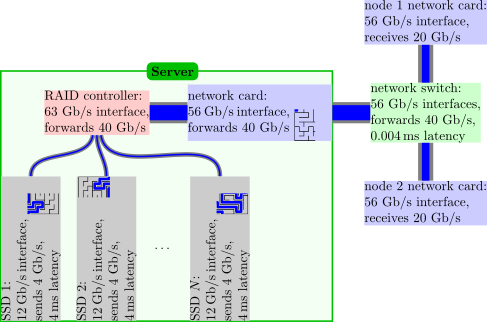
Consider the Best Way to Transfer Data
If you are transferring large amounts of data you will need to think about what may affect your transfer performance. It is always useful to run some tests that you can use to extrapolate how long it will take to transfer your data.
Say you have a “data” folder containing 10,000 or so files, a healthy mix of small and large ASCII and binary data. Which of the following would be the best way to transfer them to Comet?
scp -r data user@comet.ncl.ac.uk:~/rsync -ra data user@comet.ncl.ac.uk:~/rsync -raz data user@comet.ncl.ac.uk:~/-
tar -cvf data.tar data;rsync -raz data.tar user@comet.ncl.ac.uk:~/ -
tar -cvzf data.tar.gz data;rsync -ra data.tar.gz user@comet.ncl.ac.uk:~/
-
scpwill recursively copy the directory. This works, but without compression. -
rsync -raworks likescp -r, but preserves file information like creation times. This is marginally better. -
rsync -razadds compression, which will save some bandwidth. If you have a strong CPU at both ends of the line, and you’re on a slow network, this is a good choice. - This command first uses
tarto merge everything into a single file, thenrsync -zto transfer it with compression. With this large number of files, metadata overhead can hamper your transfer, so this is a good idea. - This command uses
tar -zto compress the archive, thenrsyncto transfer it. This may perform similarly to #4, but in most cases (for large datasets), it’s the best combination of high throughput and low latency (making the most of your time and network connection).
- Be careful how you use the login node.
- Your data on the system is your responsibility.
- Plan and test large data transfers.
- It is often best to convert many files to a single archive file before transferring.
Content from Running a parallel job (alternative episode)
Last updated on 2026-09-15 | Edit this page
ERROR
Error in `find_config()`:
! Could not find lesson configuration in any known location.
Overview
Questions
- What is the difference between array jobs and MPI?
- What benefits arise from parallel execution?
- What are the limits of gains from execution in parallel?
Objectives
- Distinguish between job arrays and MPI
- Download prime generator program
- Prepare a job submission script for the parallel executable.
- Launch jobs with parallel execution.
- Record and summarize the timing and accuracy of jobs.
- Describe the relationship between job parallelism and performance.
In the previous episode we mentioned the use of the Message Passing Interface (MPI) to accomplish parallelisation. While array jobs allow us to launch several instances of the same program, but with different data, across several nodes, MPI allows a single task to be distributed over several CPU cores.
It is thus possible to use array jobs in conjunction with MPI.
What is MPI?
The Message Passing Interface is a set of tools which allow multiple tasks running simultaneously to communicate with each other. Typically, a single executable is run multiple times, possibly on different machines, and the MPI tools are used to inform each instance of the executable about its sibling processes, and which instance it is. MPI also provides tools to allow communication between instances to coordinate work, exchange information about elements of the task, or to transfer data. An MPI instance typically has its own copy of all the local variables.
In this episode we will use two small programs, written in C, to calculate the number of primes found between two given numbers. One of the programs calculates prime and by using MPI spreads the job over several CPU cores while the other program doesn’t. After running both these programs one can compare their output to see the difference in efficiency.
If you disconnected, log back in to the cluster.
Only do this if pre-compiled binaries of the programs have not been made available to you.
Steps
- Download code
- Compile code
- Copy binaries to home directory
If you disconnected, log back in to the cluster.
Clone the repository
Compile the code.
OUTPUT
Compiling primes.c function...
Compiling single process version...
Creating executable binary...
-rwxr-x--- 1 username group 17472 Jan 23 11:14 single_gcc

Compiling primes.c function...
Compiling single process version...
Creating executable binary...
-rwxr-x--- 1 username group 7176 Jan 23 11:14 single_aocc

Compiling primes.c function...
Compiling MPI multi-process version...
Creating executable binary...
-rwxr-x--- 1 username group 17096 Jan 23 11:14 multi
Move (or copy) the binaries to your home directory
Copying the programs into your home directory
Make sure you are in your home directory.
You will need to amend the from-directory in the instruction below if you did not compile the code yourself according to the above challenge:
Help!
Many command-line programs include a “help” message. Try it with
single_gcc:
OUTPUT
You must enter two positive numbers in the range 1 - 2^32This message doesn’t tell us much about what the program does, but it does tell us that we need to provide two numbers that specify the beginning and the end of a range that lies between 1 and 2^32.
The time command
You will notice in the batch scripts that we will be creating we will
be using the time command before the name of the program.
For example:
OUTPUT
You must enter two positive numbers in the range 2 - 2^32

real	0m0.005s
user	0m0.000s
sys	0m0.002s
The very first line of the output is the output of the program we
want to run, i.e. single_gcc. After that time
returns three times. real is wall clock time. If you ran a
stopwatch, that is how long it would have taken. The user
time is the amount of CPU time it has taken. sys is
kernel/system call time. That is the time the code spent doing things
that were not part of your code, but essential stuff like interrupts,
time the kernel spent setting up processes and memory.
Running the Job on a Compute Node
Create a submission file, requesting one task on a single node, then launch it.
ERROR
Error in `snippets()`:
! snippets() called before configuration was loaded.
Use the status commands to check whether your job is running and when it ends:
Use ls to locate the output file. The -t
flag sorts in reverse-chronological order: newest first. What was the
output?
Read the Job Output
The cluster output should be written to a file in the folder you launched the job from. For example,
OUTPUT
slurm-1177272.out job_single.sh job_multi.sh single_gcc multiOUTPUT
Starting single process primes calculation (2 - 10000000)
=====================
main: Calculating primes in the range 2 - 10000000
primeCount: Calculating primes 2 - 10000000
primeCount: Found 664579 primes
main: Found a total of 664579 primes

real	0m34.476s
user	0m34.247s
sys	0m0.002s
=====================
Primes calculation complete
While MPI-aware executables can generally be run as stand-alone
programs, in order for them to run in parallel they must use an MPI
run-time environment, which is a specific implementation of the
MPI standard. To activate the MPI environment, the program
should be started via a command such as mpiexec (or
mpirun, or srun, etc. depending on the MPI
run-time you need to use), which will ensure that the appropriate
run-time support for parallelism is included.
Running the Parallel Job
The program multi uses the Message Passing Interface
(MPI) for parallelism. – this is a common tool on HPC systems.
MPI Runtime Arguments
On their own, commands such as mpiexec can take many
arguments specifying how many machines will participate in the
execution, and you might need these if you would like to run an MPI
program on your own (for example, on your laptop). In the context of a
queuing system, however, it is frequently the case that MPI run-time
will obtain the necessary parameters from the queuing system, by
examining the environment variables set when the job is launched.
Let’s modify the job script to request more cores and use the MPI run-time.
ERROR
Error in `snippets()`:
! snippets() called before configuration was loaded.Is it 16× faster?
The parallel job received 16× more processors than the serial job: does that mean it finished in 1/16th of the time?
The parallel job did take less time: 3.493s is better than 34.476s! But it is only a 9.87× improvement, not 16×.
Look at the job output:
- While “process 0” did serial work, processes 1 through 3 did their parallel work.
- While process 0 caught up on its parallel work, the rest did nothing at all.
Process 0 always has to finish its serial task before it can start on the parallel work. This sets a lower limit on the amount of time this job will take, no matter how many cores you throw at it.
This is the basic principle behind [Amdahl’s Law][amdahl], which is one way of predicting improvements in execution time for a fixed workload that can be subdivided and run in parallel to some extent.
In an HPC environment, we try to reduce the execution time for all types of jobs, and MPI is an extremely common way to combine dozens, hundreds, or thousands of CPUs into solving a single problem. To learn more about parallelization, see the parallel novice lesson lesson.
- Parallel programming allows applications to take advantage of parallel hardware.
- The queuing system facilitates executing parallel tasks.
- Performance improvements from parallel execution do not scale linearly.
Content from Running a parallel job
Last updated on 2026-09-15 | Edit this page
Overview
Questions
- How do we execute a task in parallel?
- What benefits arise from parallel execution?
- What are the limits of gains from execution in parallel?
Objectives
- Prepare a job submission script for the parallel executable.
- Launch jobs with parallel execution.
- Record and summarize the timing and accuracy of jobs.
- Describe the relationship between job parallelism and performance.
Running the Job on a Compute Node
At this point, we have installed the amdahl executable
on the system, and can now run it on the cluster.
Create a submission file, requesting one task on a single node, then launch it.
BASH
#!/bin/bash
#SBATCH --job-name solo-job
#SBATCH --partition short_free
#SBATCH -N 1
#SBATCH -n 1

# Load the computing environment we need
module load Python

# Execute the task
amdahlAs before, use the Slurm status commands to check whether your job is running and when it ends:
Use ls to locate the output file. The -t
flag sorts in reverse-chronological order: newest first. What was the
output?
The cluster output should be written to a file in the folder you launched the job from. For example,
OUTPUT
slurm-347087.out serial-job.sh amdahl LICENSE pyproject.toml README.mdOUTPUT
Doing 30.000000 seconds of 'work' on 1 processor,
which should take 30.000000 seconds with 0.800000 parallel proportion of the workload.

  Hello, World! I am process 0 of 1 on compute030. I will do all the serial 'work' for 7.021608 seconds.
  Hello, World! I am process 0 of 1 on compute030. I will do parallel 'work' for 26.302983 seconds.

Total execution time (according to rank 0): 33.326056 seconds
As we saw before, two of the amdahl program flags set
the amount of work and the proportion of that work that is parallel in
nature. Based on the output, we can see that the code uses a default of
30 seconds of work that is 80% parallel. The program ran for just over
30 seconds in total, and if we run the numbers, it is true that 20% of
it was marked ‘serial’ and 80% was ‘parallel’.
Since we only gave the job one CPU, this job wasn’t really parallel: the same processor performed the ‘serial’ work for 7.02 seconds, then the ‘parallel’ part for 26.30 seconds, and no time was saved. The cluster can do better, if we ask.
Running the Parallel Job
The amdahl program uses the Message Passing Interface
(MPI) for parallelism – this is a common tool on HPC systems.
What is MPI?
The Message Passing Interface is a set of tools which allow multiple tasks running simultaneously to communicate with each other. Typically, a single executable is run multiple times, possibly on different machines, and the MPI tools are used to inform each instance of the executable about its sibling processes, and which instance it is. MPI also provides tools to allow communication between instances to coordinate work, exchange information about elements of the task, or to transfer data. An MPI instance typically has its own copy of all the local variables.
While MPI-aware executables can generally be run as stand-alone
programs, in order for them to run in parallel they must use an MPI
run-time environment, which is a specific implementation of the
MPI standard. To activate the MPI environment, the program
should be started via a command such as mpiexec (or
mpirun, or srun, etc. depending on the MPI
run-time you need to use), which will ensure that the appropriate
run-time support for parallelism is included.
MPI Runtime Arguments
On their own, commands such as mpiexec can take many
arguments specifying how many machines will participate in the
execution, and you might need these if you would like to run an MPI
program on your own (for example, on your laptop). In the context of a
queuing system, however, it is frequently the case that MPI run-time
will obtain the necessary parameters from the queuing system, by
examining the environment variables set when the job is launched.
Let’s modify the job script to request more cores and use the MPI run-time.
BASH
[user@cometlogin01(comet) ~] cp serial-job.sh parallel-job.sh
[user@cometlogin01(comet) ~] nano parallel-job.sh
[user@cometlogin01(comet) ~] cat parallel-job.sh
BASH
#!/bin/bash
#SBATCH --job-name parallel-job
#SBATCH --partition short_free
#SBATCH -N 1
#SBATCH -n 4

# Load the computing environment we need
# (mpi4py and numpy are in SciPy-bundle)
module load Python
module load SciPy-bundle

# Execute the task
mpiexec amdahl
Then submit your job. Note that the submission command has not really changed from how we submitted the serial job: all the parallel settings are in the batch file rather than the command line.
As before, use the status commands to check when your job runs.
OUTPUT
slurm-347178.out  parallel-job.sh  amdahl   pyproject.toml
slurm-347087.out serial-job.sh LICENSE README.mdOUTPUT
Doing 30.000000 seconds of 'work' on 4 processors,
 which should take 12.000000 seconds with 0.800000 parallel proportion of the workload.

  Hello, World! I am process 0 of 4 on compute030. I will do all the serial 'work' for 6.851971 seconds.
  Hello, World! I am process 2 of 4 on compute030. I will do parallel 'work' for 6.726753 seconds.
  Hello, World! I am process 1 of 4 on compute030. I will do parallel 'work' for 6.742398 seconds.
  Hello, World! I am process 3 of 4 on compute030. I will do parallel 'work' for 6.782674 seconds.
  Hello, World! I am process 0 of 4 on compute030. I will do parallel 'work' for 6.468167 seconds.

Total execution time (according to rank 0): 13.579746 secondsIs it 4× faster?
The parallel job received 4× more processors than the serial job: does that mean it finished in ¼ the time?
The parallel job did take less time: 11 seconds is better than 30! But it is only a 2.7× improvement, not 4×.
Look at the job output:
- While “process 0” did serial work, processes 1 through 3 did their parallel work.
- While process 0 caught up on its parallel work, the rest did nothing at all.
Process 0 always has to finish its serial task before it can start on the parallel work. This sets a lower limit on the amount of time this job will take, no matter how many cores you throw at it.
This is the basic principle behind Amdahl’s Law, which is one way of predicting improvements in execution time for a fixed workload that can be subdivided and run in parallel to some extent.
How Much Does Parallel Execution Improve Performance?
In theory, dividing up a perfectly parallel calculation among n MPI processes should produce a decrease in total run time by a factor of n. As we have just seen, real programs need some time for the MPI processes to communicate and coordinate, and some types of calculations can’t be subdivided: they only run effectively on a single CPU.
Additionally, if the MPI processes operate on different physical CPUs in the computer, or across multiple compute nodes, even more time is required for communication than it takes when all processes operate on a single CPU.
In practice, it’s common to evaluate the parallelism of an MPI program by
- running the program across a range of CPU counts,
- recording the execution time on each run,
- comparing each execution time to the time when using a single CPU.
Since “more is better” – improvement is easier to interpret from increases in some quantity than decreases – comparisons are made using the speedup factor S, which is calculated as the single-CPU execution time divided by the multi-CPU execution time. For a perfectly parallel program, a plot of the speedup S versus the number of CPUs n would give a straight line, S = n.
Let’s run one more job, so we can see how close to a straight line
our amdahl code gets.
BASH
[user@cometlogin01(comet) ~] nano parallel-job.sh
[user@cometlogin01(comet) ~] cat parallel-job.sh
BASH
#!/bin/bash
#SBATCH --job-name parallel-job
#SBATCH --partition short_free
#SBATCH -N 1
#SBATCH -n 8

# Load the computing environment we need
# (mpi4py and numpy are in SciPy-bundle)
module load Python
module load SciPy-bundle

# Execute the task
mpiexec amdahl
Then submit your job. Note that the submission command has not really changed from how we submitted the serial job: all the parallel settings are in the batch file rather than the command line.
As before, use the status commands to check when your job runs.
OUTPUT
slurm-347271.out     slurm-347178.out  serial-job.sh  LICENSE         README.md
parallel-job.sh slurm-347087.out amdahl pyproject.tomlOUTPUT
Doing 30.000000 seconds of 'work' on 8 processors,
 which should take 9.000000 seconds with 0.800000 parallel proportion of the workload.

  Hello, World! I am process 4 of 8 on compute030. I will do parallel 'work' for 3.157831 seconds.
  Hello, World! I am process 0 of 8 on compute030. I will do all the serial 'work' for 6.031285 seconds.
  Hello, World! I am process 2 of 8 on compute030. I will do parallel 'work' for 3.215214 seconds.
  Hello, World! I am process 1 of 8 on compute030. I will do parallel 'work' for 3.524280 seconds.
  Hello, World! I am process 3 of 8 on compute030. I will do parallel 'work' for 3.589039 seconds.
  Hello, World! I am process 5 of 8 on compute030. I will do parallel 'work' for 3.501589 seconds.
  Hello, World! I am process 6 of 8 on compute030. I will do parallel 'work' for 3.207707 seconds.
  Hello, World! I am process 7 of 8 on compute030. I will do parallel 'work' for 3.071680 seconds.
  Hello, World! I am process 0 of 8 on compute030. I will do parallel 'work' for 3.482018 seconds.

Total execution time (according to rank 0): 9.514393 secondsNon-Linear Output
When we ran the job with 4 parallel workers, the serial job wrote its output first, then the parallel processes wrote their output, with process 0 coming in first and last.
With 8 workers, this is not the case: since the parallel workers take less time than the serial work, it is hard to say which process will write its output first, except that it will not be process 0!
Now, let’s summarize the amount of time it took each job to run:
| Number of CPUs | Runtime (sec) |
|---|---|
| 1 | 33.326056 |
| 4 | 13.579746 |
| 8 | 9.514393 |
Then, use the first row to compute speedups \(S\), using Python as a command-line calculator and the formula
\[ S(t_{n}) = \frac{t_{1}}{t_{n}} \]
BASH
[user@cometlogin01(comet) ~] for n in 33.326056 13.579746 9.514393; do python3 -c "print(33.326056 / $n)"; done| Number of CPUs | Speedup | Ideal |
|---|---|---|
| 1 | 1.0 | 1 |
| 4 | 2.45 | 4 |
| 8 | 3.50 | 8 |
The job output files have been telling us that this program is performing 80% of its work in parallel, leaving 20% to run in serial. This seems reasonably high, but our quick study of speedup shows that in order to get a 4× speedup, we have to use 8 or 9 processors in parallel. In real programs, the speedup factor is influenced by
- CPU design
- communication network between compute nodes
- MPI library implementations
- details of the MPI program itself
Using Amdahl’s Law, you can prove that with this program, it is impossible to reach 8× speedup, no matter how many processors you have on hand. Details of that analysis, with results to back it up, are left for the next class in the HPC Carpentry workshop, HPC Workflows.
In an HPC environment, we try to reduce the execution time for all types of jobs, and MPI is an extremely common way to combine dozens, hundreds, or thousands of CPUs into solving a single problem. To learn more about parallelization, see the parallel novice lesson lesson.
- Parallel programming allows applications to take advantage of parallel hardware.
- The queuing system facilitates executing parallel tasks.
- Performance improvements from parallel execution do not scale linearly.